This is part 4 of a series of guest posts by British Bondora p2p lending investor ‘ParisinGOC’. In part 1, part 2 and part 3 published in December 2014 you could read how he used the data to built decision trees to identify lending opportunities. Now you can read how that strategy worked out.

Introduction

In August 2014, I realised my portfolio of P2P loans at Bondora was not performing as I would wish. There was an urgent need to change the way I selected loans in which to invest the money I had at my disposal. My search for a better way of selecting loans lead me to use Decision Trees to analyse the loan data available from Bondora using “RapidMiner” – software available to download for free.

It is now over 6 months since I described my original work to construct the Trees. This follow-up article chronicles what I believe is the success of my efforts to date whilst also describing the multiple factors, both within and beyond my control, that mean that, whilst I feel very comfortable with the progress made to date, others may feel that I have just been lucky!

The journey since I created my first Decision Tree and started to make purchasing decisions based almost totally on their outputs has been one of constant change. Detailing the changes to elements over which I have no control has shown me how they contribute to what I believe is success as much as my own efforts to improve the selection processes. Describing the change in the Decision Trees as well as their use in the dynamic Bondora environment has left me feeling that, without constant monitoring and review of both the process of creating the Trees as well as their use, it may still be very easy to snatch defeat from the jaws of victory.

Key to ensuring the veracity of my protestations of success has been the maintenance of a consistent approach to my selection and lending process. To this end, I will describe those changes to my process that I can control and explain how and why such changes have taken place. In short, I have maintained a restricted buying policy, investing only the minimum amount (5 Euros) at any one time and, latterly, only buying a maximum of 2 loan parts (of 5 Euros each) in any one loan, depending on the outputs from the Decision Trees and my own mood at the moment of purchase.
I realise that this last phrase is not at all scientific, but the fact that my Portfolio of c.12000 Euros was not performing as expected was for me, a non-trivial affair and some emotional response has to be accommodated.

I have already stated that I believe my efforts have been successful. This is based on the fact that the rate of default (Once a loan principal has been overdue for 60+ days, it is labelled as “defaulted” – Bondora FAQ) in my portfolio has returned to historical, pre-2014 levels. Up to this time, even though I had come to realise that I needed to actively manage my portfolio, my selection of loans was done almost entirely using the “Portfolio Manager” – an automated, parameter-driven purchasing function provided by Bondora and supplemented by instinctual analysis of the descriptions of the Loan Applications available to invest in.

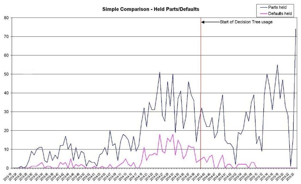
Looking at the simple chart of Held Parts/Defaults, the number of defaults in held loans rose significantly over the summer of 2014, coinciding with a big increase in both the number and value of investments on my part. Referring to the same chart, it can be seen that, even though the number of investments remains close to summer 2014 levels, my defaults have fallen to the numbers experienced earlier, at much lower volumes.

With my new-found confidence that I have a process for selection and management that appears to be sound, I have started to increase the volume of Loan Parts purchased so that the value is now approaching Summer 2014 levels of investment.

Progress to date

Graphical representation of Progress

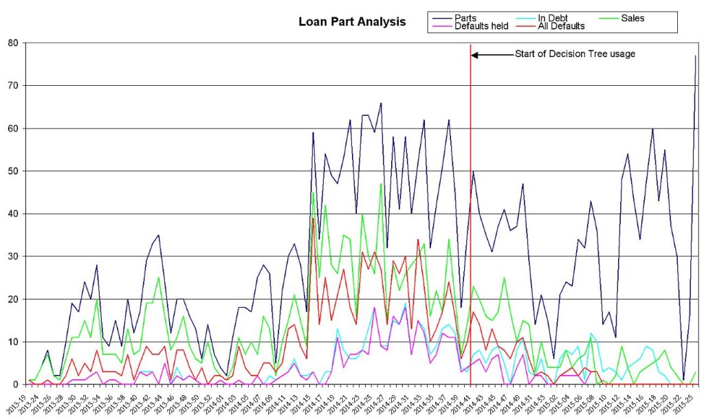
I will use a more detailed graph showing the volume of Loan Parts purchased, those subsequently sold, those “Overdue” and those in default (still held by me as well as sold) to hopefully illustrate the performance of my selection and management processes.

The chart is quite “busy” and probably merits some detailed explanation. All data relating to a loan is “anchored” on the week of purchase. Thus, a week number shows volumes of Loan Parts purchased that week as well the number of those same loans that were then sold, the number that went on to default (whether still in my possession or not), the number “In Debt” (as at 20th June, 2015, the date of the data download) and finally, the number of defaults still held by me.

From the graph, it is clear how I expanded my portfolio from initial, tentative purchases in midsummer 2013 through larger volumes purchased through the summer of 2014 as I invested more cash on top of income from previous loans. This increase in purchases stops suddenly in weeks 37 to 39 (mid- to late-September 2014) as I realised all was not going as well as I had intended.

Since the end of September 2014, all my purchases were made using only income earned from previous investments. My cash reserves built up from 1st October 2014 onwards as my restricted purchasing regime (detailed below) did not use all my income from previous investments. This cash reserve is now reducing as I have increased my purchasing activity (also detailed below) as the success of my efforts has materialised.

Returning to the chart, it should be noted that the “In Debt” numbers are, as stated earlier, as at 20th June 2015. Hence the almost total historical correlation between this figure and the defaults held. As the graph moves closer to the present day, this correlation becomes weaker as the loan has not yet had enough time to default, should that be its final destination.

This is demonstrated by the total lack of defaults since week 9 (last week in March) of this year. Loans purchased subsequently have not yet had time to default; yet the numbers “In Debt” remain high. A proportion of the Loans “In Debt” will be sold, possibly at a significant discount if necessary.
My personal goals for my portfolio are subject to a deadline and I wish to minimise the number of defaulted loans I hold, even where this incurs a greater potential loss than just holding on to them and hoping for some return over an unknown timescale. I therefore attempt to sell almost every loan part that is showing signs of stress, as demonstrated in the extreme by default! So it is that I have sold well over half the loans I have ever purchased before September 2014.

Whilst impending default is the extreme example of why I may sell a loan, I commence tight management of any loan part on the day a payment is due, sometimes pre-empting the Bondora indicator (which is triggered on midnight of the day due). By realizing the available profit, I am making the conscious decision to attempt to take the profit that is available to me at the point where a loan part is showing some stress and will try harder to sell the loan the more stress it displays. Whilst this may sometimes incur a significant loss, I have made an overall profit on loan parts sold, including earned interest but less all costs. This profit counts the interest earned on sales that were sold, possibly at a discount, so there is a danger of counting this interest twice, which is why this analysis deals only with volumes of loan parts, not value.

I have included numbers for sales and sold defaulted parts for completeness. This is a review of my selection process (the use of Decision Trees) not my overall management strategy. I therefore feel that the inclusion of all outcomes resulting from the initial purchase is necessary.

When analysing the numbers represented on the chart, I am acutely aware that I keep referring to historical default rates”. In truth, the default rate (all defaults) of my purchases has never been truly low! In the article about the creation of the Decision Trees, I revealed that I used to work for a major UK Bank and, in this context I feel that default rates of 3%+ are high. Looking at the graph of my portfolio performance, my rate of all defaults has always been dreadful – cumulatively 25% throughout 2013, rising to 38% at its nadir in the summer of 2014 and falling back to 33% as at week 9 of 2015. My assertion that using Decision Trees to select loans has been a success stems from the fact that the comparative cumulative default rate from 1st October 2014 (week 41) to 2015 week 9 is “only” 20% compared with the 33% historical rate shown above.

The comparative numbers for held defaults (i.e. not sold) are 18% over 2013 rising to 31% in summer 2014 then falling to 25% at 2015 week 9. For the period of Decision Tree usage alone, the figure is 13%. This final figure is notable as I select loans that, according to the Decision Trees, show an historical default rate lower than 5% to 7%. So, if nothing else, I have undoubtedly proved the mantra of investment organisations the world over, namely: “Past performance does not guarantee future results.” (Bondora, General statistics note).

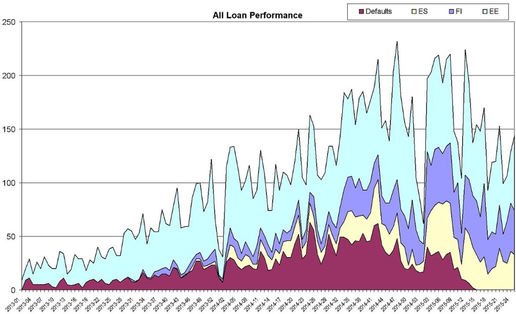
I have kept my own analysis somewhat self-referential as I care not about the overall Bondora default rate whilst my own performance is not up to scratch. For completeness, I have done a fairly rough-and-ready analysis of the full Bondora book for the same period (early 2013 to date), just to see if the use of the Decision Trees is indeed producing what could be termed better than average results.

This chart (using the Loan Date as the only date reference, as with my own data) shows the defaults across all countries with the individual country volumes stacked on top. In terms of real numbers, at worst (including parts I have sold) my performance over 2013 was marginally worse than average – 25% against the average across the book of 23%. This worsened dramatically during 2014 to peak at 38% cumulatively at weeks 32/33 compared with the average across the book of 26%. This is the point at which I realised things were not going well!

Compared with the cumulative average across the book of 23.69%, my cumulative average has reduced to a “worst view” still at 33%! This outcome looks a lot better for me when compared only with the actual Loan Parts that I still hold, when the comparative figures are a peak of 31% in weeks 38/39 of 2014 reducing to 25% at week 9 of 2015 – only marginally worse than the average for the book as a whole.

If I now compare performance across the book to my own performance since week 41 of 2014, the cumulative default rate across the whole book for the 22 weeks 2014-41 to 2015-09 is 18.74%. My “worst case” view is 20%, suggesting that the use of the Decision Trees analysis is slightly worse than if one could buy a single example of every loan available. However, I am not just buying and holding. My management of my holdings reduces my actual default rate to 13%, lower than at any point during my investing at Bondora. It also shows that I was right to change my strategy after the summer of 2014, as my own performance over that summer was significantly worse than the average across the book although my earlier performance through 2013 and early 2014 was (IMHO) creditable.

Continue reading in part 5!